Carl Malings
New member
Hello all,
At the end of Part 2 of our training, I encouraged everyone to use some of the resources mentioned during the training (especially NASA Worldview and NASA Giovanni) to look at satellite air quality data products for their region of interest, and if they found something interesting, to post it to this forum. As an example, I took a quick look at the area where I live and work (the NASA Goddard Space Flight Center in Greenbelt, Maryland).
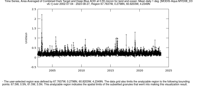
I started by using NASA Giovanni to examine the time series of satellite AOD from the MODIS-Aqua instrument, focusing into my area of interest, and making a time series plot of the Monthly average values from the MYD08_M3 Level 3 data product:
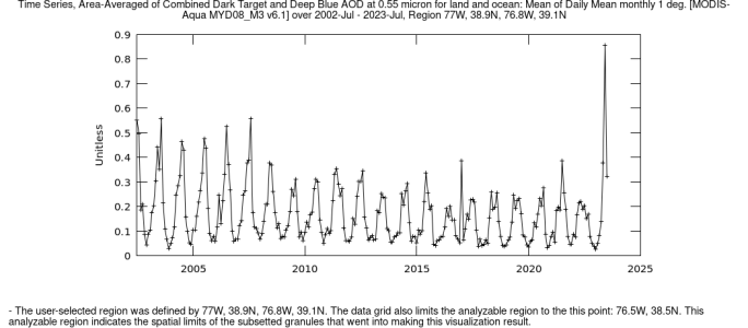
It’s important to note that, although I defined a small bounding box around my area of interest, the resolution of the data is actually coarser, so I am getting a one-degree grid-box average which includes my location of interest, and not necessarily what is happening exactly in my selected area; there is a disclaimer to this effect at the bottom of the plot.
You can see a general trend of decreasing AOD over time, although this is masked by the larger variability due to seasonal cycles. You can also see the very high AOD in June of 2023, which had a higher average than any other month in the data record; this corresponds to the wildfire smoke event which impacted Eastern Canada and the Northeastern US, which I mentioned a few times during the training. Here’s another visualization of that event, using geostationary data from the GOES-East satellite in NASA Worldview:
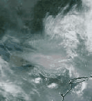
You can see how the prevailing wind patterns moved the smoke south from its origins to blanket much of the Northeastern US, including Greenbelt. I created this GIF using NASA Worldview; I didn’t get a chance to go over this functionality during the training but there is a HAQAST Tutorial which covers how to save screenshots and animations from Worldview. You can also share links directly to visualizations in Worldview, once you have them set up the way you want; for example, here is a link to the setup which I used to create that GIF:
https://worldview.earthdata.nasa.go...Color(hidden)&lg=true&t=2023-06-06-T16:01:39Z
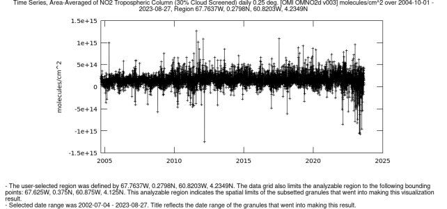
Going back to NSA Giovanni, I also looked at the OMI NO2 data record for my area of interest (this time, as a time series of the daily concentrations):
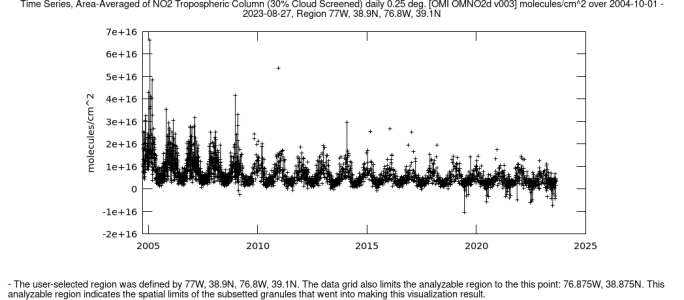
Again, you can see the general trend of decreasing concentrations over time, as well as some seasonal variability in concentrations. This time you don’t see the strong signal in June 2023 from the wildfire smoke, since NO2 is less likely to be transported far from its origins, and likely wouldn’t show up so far away from the fires. Something worth noting here is that some of the values on this plot are negative. In reality, it is impossible to have a negative concentration of NO2 in the atmosphere; however, the satellite retrievals of column NO2 are imperfect, and sometimes the outputs are negative. Typically, we recommend not to remove these negative values from the dataset; that’s because, when averaging over a long time series, these negative errors will balance out positive errors at other times, and lead to a better average value than you would have obtained if you had first removed the negative values.
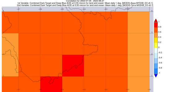
Finally, I wanted to show another kind of analysis which can be done in NASA Giovanni: a correlation plot. These can be used to show the correlation (or the strength of the linear relationship) between two datasets. In this case, I am comparing the MODIS-Aqua and MODIS-Terra AOD datasets. Recall from the training that these two satellites pass over at different times of day. By correlating these two datasets, I can assess how AOD might change throughout the day (at least at between the two times of day when the satellites pass overhead). A strong correlation would indicate that day-to-day changes in AOD are a larger contributor to AOD variability than changes during the day. A weak correlation indicates that AOD changes between these two times of day are similar to or greater than day-to-day changes. This might give me a sense of what could be driving these changes as well. For this example, I am shifting my analysis period (to focus on the calendar year of 2022) and my analysis domain (to the contiguous US).
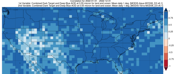
You can see in the figure that in most areas of the Eastern and Northwestern US, the correlations are high, indicating that day-to-day changes seem to be the primary driver for AOD variability. However, over the Southwestern US, the correlation is weaker, indicating that hour-to-hour changes in AOD may be the driving factor there. This might indicate that, while polar-orbiting instruments (with about one observation per day) are probably sufficient to capture the variability in AOD for the Eastern US, for the Western US, it might be beneficial to take a closer look at what geostationary satellite AOD can tell us about hour-to-hour changes, as these can be a driving factor for AOD variability in some areas.
Again, this was a very quick analysis of the data, and more work would be needed to draw firm conclusions, but hopefully this can give you an idea of how you might be able to use tools like Worldview and Giovanni to do exploratory analysis of relevant satellite data for your applications of interest.
- Carl
At the end of Part 2 of our training, I encouraged everyone to use some of the resources mentioned during the training (especially NASA Worldview and NASA Giovanni) to look at satellite air quality data products for their region of interest, and if they found something interesting, to post it to this forum. As an example, I took a quick look at the area where I live and work (the NASA Goddard Space Flight Center in Greenbelt, Maryland).
I started by using NASA Giovanni to examine the time series of satellite AOD from the MODIS-Aqua instrument, focusing into my area of interest, and making a time series plot of the Monthly average values from the MYD08_M3 Level 3 data product:

It’s important to note that, although I defined a small bounding box around my area of interest, the resolution of the data is actually coarser, so I am getting a one-degree grid-box average which includes my location of interest, and not necessarily what is happening exactly in my selected area; there is a disclaimer to this effect at the bottom of the plot.
You can see a general trend of decreasing AOD over time, although this is masked by the larger variability due to seasonal cycles. You can also see the very high AOD in June of 2023, which had a higher average than any other month in the data record; this corresponds to the wildfire smoke event which impacted Eastern Canada and the Northeastern US, which I mentioned a few times during the training. Here’s another visualization of that event, using geostationary data from the GOES-East satellite in NASA Worldview:

You can see how the prevailing wind patterns moved the smoke south from its origins to blanket much of the Northeastern US, including Greenbelt. I created this GIF using NASA Worldview; I didn’t get a chance to go over this functionality during the training but there is a HAQAST Tutorial which covers how to save screenshots and animations from Worldview. You can also share links directly to visualizations in Worldview, once you have them set up the way you want; for example, here is a link to the setup which I used to create that GIF:
https://worldview.earthdata.nasa.go...Color(hidden)&lg=true&t=2023-06-06-T16:01:39Z
Going back to NSA Giovanni, I also looked at the OMI NO2 data record for my area of interest (this time, as a time series of the daily concentrations):

Again, you can see the general trend of decreasing concentrations over time, as well as some seasonal variability in concentrations. This time you don’t see the strong signal in June 2023 from the wildfire smoke, since NO2 is less likely to be transported far from its origins, and likely wouldn’t show up so far away from the fires. Something worth noting here is that some of the values on this plot are negative. In reality, it is impossible to have a negative concentration of NO2 in the atmosphere; however, the satellite retrievals of column NO2 are imperfect, and sometimes the outputs are negative. Typically, we recommend not to remove these negative values from the dataset; that’s because, when averaging over a long time series, these negative errors will balance out positive errors at other times, and lead to a better average value than you would have obtained if you had first removed the negative values.
Finally, I wanted to show another kind of analysis which can be done in NASA Giovanni: a correlation plot. These can be used to show the correlation (or the strength of the linear relationship) between two datasets. In this case, I am comparing the MODIS-Aqua and MODIS-Terra AOD datasets. Recall from the training that these two satellites pass over at different times of day. By correlating these two datasets, I can assess how AOD might change throughout the day (at least at between the two times of day when the satellites pass overhead). A strong correlation would indicate that day-to-day changes in AOD are a larger contributor to AOD variability than changes during the day. A weak correlation indicates that AOD changes between these two times of day are similar to or greater than day-to-day changes. This might give me a sense of what could be driving these changes as well. For this example, I am shifting my analysis period (to focus on the calendar year of 2022) and my analysis domain (to the contiguous US).

You can see in the figure that in most areas of the Eastern and Northwestern US, the correlations are high, indicating that day-to-day changes seem to be the primary driver for AOD variability. However, over the Southwestern US, the correlation is weaker, indicating that hour-to-hour changes in AOD may be the driving factor there. This might indicate that, while polar-orbiting instruments (with about one observation per day) are probably sufficient to capture the variability in AOD for the Eastern US, for the Western US, it might be beneficial to take a closer look at what geostationary satellite AOD can tell us about hour-to-hour changes, as these can be a driving factor for AOD variability in some areas.
Again, this was a very quick analysis of the data, and more work would be needed to draw firm conclusions, but hopefully this can give you an idea of how you might be able to use tools like Worldview and Giovanni to do exploratory analysis of relevant satellite data for your applications of interest.
- Carl


